GROUP = Type_Calculation:  type, total_solutes, total_grids

• type [string] (sda_2proteins) : type of calculation - defines which type of calculation will be performed. The following options are available:
  • sda_2proteins : for docking, association rate calculation or electron transfer
  • sdamm : simulation with multiple proteins.
  • sda_koff : k_off calculation.
  • sda_energy : compute interaction energy from complexes or trajectory files.
• total_solutes [integer] (2) : total number of solutes
• total_grids [integer] (2) : total number of grids (if a solute has more than one grid to account for conformational/structural variation, this only counts as 1 grid ). In fact, the number of set_of_grids = number of GROUP Solute_Grid

GROUP = Reaction Criteria:   computation, rxna12f, et_sol1, et_sol2, dind, nnnons, nwrec, sdamd

• computation [string] (off_rc) : define which type of simulation is being performed. Options:
  • association : compute association rate at every distance and for any number of contacts defined in group RateCalculation. Use *.rxna file and dind to define the criteria and their independence, all criteria are considered as nonspecific.
  • docking : a complex must satisfy all specific criteria and at least nnnons non-specific ones in order to be saved in the complexes file
  • electron_transfer : compute elctron transfer. The reaction criteria are read from 2 input files ( et_sol1 and et_sol2 )
  • all : all complexes are saved to the complexes file. No checks are performed
  • off_rc : disactivate the reaction criteria module, no calculations performed
• rxna12f [string] (p12.rxna) : filename for the reaction criteria used for docking or association rate calculations.
  Input examples for barnase-barstar docking and association rates are available in the examples. Reaction atoms do not have to be real atoms, although in this file these atoms/points should be given like atoms in PDB format.  Different combinations of the same atoms/points can be prepared by editing these reaction atom files
• et_sol1, et_sol2 [string] (empty) : filenames for the reaction criteria for electron transfer calculations.
• dind [float] (6.) : minimal distance (in Å) between atoms on the same solute defining contacts for satisfying reaction criteria (equivalent to d_min in figure below)
• nnnons [integer] (2) : minimum number of nonspecific constraints to satisfy to define an encounter complex
• nwrec [integer] (0) : number of the window up to which the complexes are recorded.  For example, in the situation below, nwin=5 reaction distance windows are defined, and rates for forming contacts at each of these 5 distances will be monitored.  Encounter complexes with contact distances less than win0+dwin*(nwrec-1), will be recorded.
• sdamd [integer] (0) : flag to activate the option of recording encounter complexes at the windows distance according to win0+dwin*(nwrec-1).  For example, in the case where win0=4.0, nwrec=23, encounter complexes will be recorded with at least one reaction contact at a distance of 15A.

Reaction criteria are used to define a "complex" between 2 solutes. Full freedom is let to the user:

• Define a center-to-center distance criteria between the solutes, usually for docking
• A set of donor-acceptor pairs from an initial complex, needed for association rates
• Any other constraints suitable with experimental data: distance between 2 atoms satisfying crosslink experiments, FRAP or FRET data, known interactions with a specific residue / ligand...
• All constraints can be freely combined

The list of reaction criteria must be provided in a separate file (conventionally named with a suffix *.rxna), where the fields indicate:

• The keyword for the type of reaction criteria (discussed below)
• The position of the atom of the solute 1 (the atom number is needed in the case of a flexible solute)
• The minimum distance that the 2 reaction criteria must satisfy
• The position of the atom of the solute 2 (the atom number is needed in the case of a flexible solute)

For docking, there are 3 different types of reaction you can use:

• CSPEC: specific constraint, this reaction criterion must be satisfied for the complex to be accepted
• CNONS: nonspecific constraint, at least nnnons of these reaction criteria must be satisfied
• ASPEC: anti-specific, this criterion must be invalid (new in SDA 7)

For association rate calculations, all entries in the *.rxna file are considered as CNONS. But you can still record complexes and adjust the nwrec input parameter.

To get the specific format of the *.rxna file, we advise you to look at the input files in the barnase-barstar example of docking. Here are illustrated:

• A blind simulation, where only the center to center distance between the protein is used as a criterion
• An example where the center-to-center distance criterion is used together with nonspecific reaction criteria

Or you can refer to the technical documentation, linked here in the section Reaction Criteria.
(The doxygen documentation must be generated before using this link).

Usage of dind
To avoid an artificially large number of contacts, the variable dind can be used.
On the figure below, all atoms used in the reaction criteria are represented by spheres. But only those which are at a separation greater than d_min are considered as independent (black spheres). So with this schema, there will be a maximum of 4 independent contacts.

GROUP = RateCalculation:  win0, nwin, dwin, nb_contact, bootstrap, fpt, stop_traj,analytical_correction

Calculate bimolecular association rate constants using the Northrup, Allison and McCammon method (see Northrup, Allison McCammon, (1984), J. Chem. Phys.).

• win0 [float] (3.0) : reaction distance window minimum value (in Å)
• nwin [integer] (0) : number of reaction distance windows.
• dwin [float] (0.5) : reaction distance window step (in Å).
• 
• nb_contact [integer] (4) : maximum number of pair contacts to be considered. This parameter is only applicable for association rate calculations.
• bootstrap [bool] (0) : if 1, association rates and first passage time results are printed for every trajectory. Final results can be computed with bootstraping (auxi/Bootstrap_multiCPU.py)
• fpt [bool] (0) if 1, record the first passage time, if bootstrap==1 same processing with (auxi/bootstrap.py)
• stop_traj [bool] (0) if 1, simulated trajectories will stop when the most strict reaction criteria definition is met (i.e. greatest number of contacts at the closest distance window). This may speed up your simulations, particularly in the case of strongly interacting simulations, although this will depend strongly on your choices of nb_contact and win0.
• analytical_correction [bool] (0) if 1, the analytical correction for centrosymmetric forces is computed for estimating the bimolecular association rate constant with the Northrup, Allison and McCammon method . When using this option, it is required that the interaction potential is centrosymmetric at the b surface, but it can be non-zero. This option requires that the real_net_charge and dh_radius is set for all solutes in the solute grid groups of the input file, and that the ionic_strength is set in the analytical group. If 0, there must be no interaction forces between the solutes at a separation of start_pos

GROUP = Analytical:  h_analytic, debyeh, ionic_strength, hydrodynamic, disable_normal_hi, disable_image_hi, disable_height_hi, surface_height, hom_charged_surf, surface_fact, gouy_chapman

• h_analytic [float] (0.01) : defines the bin size (in Å) of the arrays of the precomputed debye-hueckel values.
• debyeh [bool] (0) : if 1, activates Debye-Hueckel interactions for all solutes
• dh_imgchg [bool] (0) : if 1 and a surface is present, the image-charge model used for modelling electrostatic interactions with conducting surfaces is extended to use debye-huckel interactions for all solutes whose images lie outside of their electrostatic grids.
• ionic_strength [float] (0.150) : if Debye-Hueckel computed, specifies the ionic strength (in Molar)
• hydrodynamic [bool] (0) : if 1, activates mean-field hydrodynamics interactions for all solutes. If a surface is present in the simulation then surface effects will be included. This can be disabled with the options disable_normal_hi, disable_image_hi and disable_height_hi. These options are meant for investigating the effects of hydrodynamic interactions of various types, and for debugging. In most cases all hydrodynamic components should be included.
• disable_normal_hi [bool] (0) : if a surface is present and this option is set to 1, normal mean-field hydrodynamics interactions between solutes are disabled.
• disable_image_hi [bool] (0) : if a surface is present and this option is set to 1, mean-field hydrodynamics interactions between solutes and their surface reflected images are disabled.
• disable_height_hi [bool] (0) : if a surface is present and this option is set to 1, the height dependent slowdown in diffusion close to the surface is disabled.
• lvol_rcut [float] (0.0) : defines the local volume radius if hydrodynamics interactions are used. Must be greater than the largest vol_radius of any solute in the system.
• surface_height [float] (0.0) : defines the height in Angstroms above a surface at which the image method is applied for surface hydrodynamic interactions. Typical value used in the Lysozyme_mica example is 2.0.
• hom_charged_surf [bool] (0) : if 1, the long-range Debye-Hückel electrostatic treatment for a surface is activated
• surface_fact [float] (0.0) : defines the prefactor for the surface charge potential (1.0 = (infinitely) thick surface (default for the Lysozyme_mica example); 0.5 = thin surface, e.g. represented by one atom layer
• gouy_chapman [bool] (0) : if 1, use Gouy-Chapman treatment instead of Debye-Huckel for the long range electrostatics of the Surface. The Gouy-Chapman treatment is the solution to the non-linearized Poisson-Boltzmann equation for a wall-geometry, whereas the Debye-Huckel treatment models the linearized Poisson-Boltzmann equation.
• surface_fact [float] (0.0) : defines the prefactor for the surface charge potential (1.0 = (infinitely) thick surface (default for the Lysozyme_mica example); 0.5 = thin surface, e.g. represented by one atom layer

GROUP = Solute_Grid: nb_solute, pdb_filename, diffusion_trans, diffusion_rotat, real_net_charge, surface_charge_dens, rotate, surface, flex, epf, qef, edf, hdf, ljf, lj_repf, nb_lj, atom_lj, list_conformation, dh_radius, vol_radius, total_conf, method, initial_conf, frequency, std_frequency, surface_charge_dens

• nb_solute [integer] (1) : number of identical solutes ( of the same type)
• pdb_filename [string] (empty) : name of pdb file for this group of solutes
• diffusion_trans [float] (0.0123) : absolute translational diffusion coefficient in Ų/ps. In the case of sda_2proteins, the translational diffusion constant of solute 2 should be assigned as the sum of the diffusion coefficients of solute 1 + solute 2 to simulate the relative translational diffusion.
  According to the Einstein-Stokes formula, the translational diffusion constant scales inverse proportionally to the solvent viscosity (which itself has a complicated dependence on the temperature), and inverse proportionally to the (hydrodynamic) radius of a solute. 1 Ų/ps = 10^-8 m²/s = 10^-4 cm²/s
• diffusion_rotat [float] (1.36e-4) : rotational diffusion coefficient of the solute in radian²/ps. This is inversely proportional to the square of the solute radius.  diffusional_rotat is inversely proportional to the solvent viscosity. For lysozyme, for example, dr=2.6*10^-5 radian²/ps.
• real_net_charge [float] 0.0 : Total net formal charge on the solute. Note that this is generally different to the sum of the effective charges which are used in calculating electrostatic forces and energies via interaction with Poisson-Boltzmann derived potential grids.   The charges set here are used to approximate long range charge interactions between solutes using a Debye-Hueckel sphere approximation, if debye is set in the Analytical group, and in the analytical correction to the rate constant calculations, if analytical_correction is set in the RateCalculation group.
• surface_charge_dens [float] (0.0) : If the solute is a surface, this option can be used to define an average charge density for surface. The interaction with other solutes is then modelled using a Debye-Hueckel sphere approximation where spherical charge solutes interact with a homogeneously charged surface. If an electrostatic grid is included in this Solute_Grid group, then the approximatation is made in regions outside the grid. With this option ionic_strength must be set in the Analytical group. Unit is in e/Angstrom**2
• rotate [bool] (1) : switch to define whether the solute rotates. 0 means no rotation and diffusion_rotat is not used. 1 means the solute can rotate and diffusion_rotat is used.
• surface [bool] (0) : switch to define whether this solute is a surface. Being treated as a surface will influence the distance computation and periodic boundary conditions, and rotate will be set to 0 for this solute
• vert_excl [bool] (0) : if set to 1 in the Solute_grid group of the central solute in a bimolecular simulation, the minimum solute separation at which it is assumed safe to ignore checks for excluded volume violations depends only the z coordinate of mobile solute, rather than the centre-to-centre distance. This is always assumed if the central solute is defined as a surface.
• xcent, ycent, zcent [float] (geometric centre of solute) : options to set the centre point of the central solute in a bimolecular simulation. The coordinates should be defined in the coordinate frame of the input PDB file. If not present in the input file then the geometric centre of the solute is used. This centre point is used to define the location of the starting and ending points of the trajectories (defined by start_pos and c in the geometry group. This can be useful in the case of a surface, or otherwise non-spherical solute, as it allows the simulation volume to be centred on a surface lying point. If one of these variables is set, then all must be.
• flex [bool] (0) : define if this solute(s) is flexible (i.e. has more than 1 structure/conformation) or not
• image_charge [bool] (0) : define if the electrostatic image charge of this solute(s) must be computed. It is relevant in the case that one solute is a metal surface.
• stoke_radius [float] (0.) : Obsolete: This option is now replaced by the radii options shown below.
• dh_radius [float] (0.) : if > 0, indicates the radius used to represent the solute cavity in the Debye-Hueckel sphere charge model.
• This option can be used as a long range correction to the truncation of electrostatic grids in all-atom simulations, and in coarse-grained sphere simulations and adaptive-resolution crowder simulations.
• vol_radius [float] (0.) : if > 0, indicates the radius used for calculating the local occupied volume fractions of the mean-field hydrodynamic interaction model.
• Hydrodynamic interactions are implemented with the Weinstein method, where the diffusion coefficients are rescaled during the trajectory depending on the instantaneous local volume fraction of solutes around one solute. The infinite dilution values of the diffusion coefficients can be obtained from the HYDROPRO program, for instance, or determined from experiments. See Mereghetti et al. (2012)in references
• epf [string] (empty) : filename for the electrostatic potential of the solute in UHBD binary format.  It is assumed that the potentials are written in kcal/mol/e units.  Note that APBS generated grids written in UHBD format are in units of kT/e and ascii and as such cannot be used directly with SDA.  They should be rescaled and converted with the auxiliary program convert_grid, to bring them into consistency with UHBD format.
• qef [string] (empty) : filename for effective charges of the solute. This is the output of the ECM suite program.  See detailed description in the faq
• edf [string] (empty) : filename for the electrostatic desolvation potential of the solute in UHBD format. This grid can be calculated with the program make_epedhdlj_grd which is included in the SDA distribution (units in kcal/mol/e).
• hdf [string] (empty) : filename for the hydrophobic desolvation potential of the solute in UHBD format. This grid can be calculated with the program make_epedhdlj_grd which is included in the SDA distribution.
• lj_repf [string] (empty) : filename for the soft-core repulsion (approx. repulsive term of Lennard-Jones) grid of the solute in UHBD format. It is intended to be used with sdamm only where it replaces the use of the exclusion grid. This grid can be calculated with the program make_epedhdlj_grd which is included in the SDA distribution.
• nb_lj [integer] (0) : define the number of Lennard-Jones potential grids. Used for the implementation of the ProMetCS force field.
• ljf [array of string] (empty) : filenames for the Lennard-Jones potential grids of the solute in UHBD format. This grid needs an additional tool to be computed
• atom_lj [array of string] (empty) : atom names for the Lennard-Jones interactions. If an unusual atom name, use the "add_atoms" file to define the sites of interaction.
• These variables are only needed in the case where the flag flex is set to 1
• list_conformation [string] (empty) : filename of the file which defines multiple conformations/structures for a solute. Every GROUP SoluteGrid may have a different list.
• total_conf [integer] (0) : define the total number of conformations/structures, if this solute is treated as flexible
• method [string] (empty) : choose between the methods implemented for changing conformations/structures. Available options are:
• • random : Choose a random conformation (depending on nearest input). The same conformation can be chosen. Energies are not evaluated
  • minimum : Implemented only with nearest=1. The minimum energy between the actual and the closest conformations (1 or 2 ) is selected
  • metropolis : The potential energy in the initial conformation (E0) is computed. For a random chosen conformation ( depending on nearest ), the new energy (E1) is computed and the move is accepted if:
  • • the new conformation has a lower energy: E1 is less than E0, or
    • a random number uniformly generated in the range [0,1] is lower than exp(E1-E0)
• nearest [bool] (0) : If 1, moves are limited to the nearest neighbour ( conformation +/- 1). It is used with conformations from normal mode analysis for instance.
  Otherwise a random conformation is chosen (used with NMR structures). The same conformation can be selected.
• initial_conf [integer] (1) : Specify the conformation chosen at the beginning of every trajectory.
  -1 makes a random choice
• frequency [float] (100) : Specify the delay between the changes in conformation (in ps). The delay is computed as a Gaussian random number with average frequency and standard deviation std_frequency.
• std_frequency [float] (0) : Specify the standard deviation (in ps). Used in the case of SDAMM to avoid synchronisation between the solutes.

GROUP = Geometry:   type, pbc, surface, escape, start_position, c_surface, min_X, max_X

• type [string] (sphere) : specify the geometry of the simulation box
• sphere : : Use a spherical geometry, only for use with sda_2proteins types of simulation
• box : : Use a box for simulation, only for use with sda_2proteins types of simulation (protein-surface case) and with sdamm
• pbc [bool] (0) : Switch on Periodic Boundary Conditions. Apply only with a box geometry
• surface [bool] (0) : Indicates if a surface is present in the system. PBC rules are modified in this case. Can also be used with a spherical geometry in sda_2proteins simulations
• escape [bool] (1) : Indicates if a solute can escape. The trajectory is then stopped when the solute reaches the c_surface (with a sphere) or zmax (in a box)
• start_pos [float] (100.) : Indicates the initial position (in Å) of the second solute in sda_2proteins. Simulations are started by placing the center of the second solute at the distance start_pos .  This corresponds to the b-surface for a spherical geometry.
  If surface is activated, the initial position is generated on the upper-half of the sphere.
  For calculation of association constants, there should be no interaction between the solutes at this distance if analytical_correction = 0, or the interaction should be centrosymmetric if analytical_correction = 1. To ensure there are no grid-based interactions at this distance, start_position can be selected to be larger than the sum of the solute 1 (or 2) grid extents and the solute 2 (or 1) radius.
  To check with box.
• c [float] (150.) : defines the c-surface (in Å) in the case of a sphere
• <X>min,<X>max [float] (0.) : where <X> = x, y or z. Defines the size of the box (in Å). If escape is activated, zmax has the role of the c-surface.
• half_sphere [bool] (0) : Replace the spherical b surface with a spherical cap surface above an xy plane at a height z = min_height. This option is always used in the presence of a surface.
• min_height [float] (0.0) : defines the height of the spherical cap, relative to the centre of the centre solute, when option half_sphere is used.

Typical setup for simulations within a sphere. Trajectories are started at the b-surface (start_pos) and finish when solute 2 goes through the c-surface (c).

GROUP = Timestep:  variable,dt1, swd1, dt2, swd2

• variable [bool] (1) : switch to a variable timestep ( in sda_2proteins simulation), or to a fixed timestep (sdamm) when the value of dt1 is used
• dt1 [float] (1.0) : basal simulation timestep (in ps, picoseconds).  This is the smallest timestep used and is employed when the center-to-center separation is less than swd1 or the distance at which the solutes have the possibility to contact (i.e. the center-to-center distance between solutes is less than rhit = the sum of maximal extents + probe radius + maximal radius of solute 1 atoms).
• swd1 [float] (50.0) : center-to-center distance (Å) at which the timestep starts to increase
• dt2 [float] (20.0) : timestep at distance swd2
• swd2 [float] (90.0) : center-to-center distance at which timestep equals dt2.
• height_dependent_dt [bool] (0) : if set to 1, the variable timestep depends on the z coordiate of the mobile solute, rather than the centre-to-centre distance between the solutes. This option is always used when a surface is present.
• rswd [*] (*) : deprecated in SDA 7, the rotation of solute2 is only proportional to the timestep

These parameters define the variable timestep designed to accelerate simulations. As shown in the figure below, the timestep is automatically decreased to zero near the c-surface to reduce artifacts due to truncation of the trajectories. Although the profile of the time step influences the computed rates, the most important parameter is dt1. Take care not to choose a too small value for this parameter (since the computing time scales almost linearly with it). The physical parameter sqrt(dt*dm) measures an average Brownian dynamics step length. This must be less than 1 Å, which is the characteristic distance describing the roughness of any protein surface since the atomic bond lengths and van der Waals radii define this scale. Moreover, dt1 should be less than the characteristic distance over which the interaction forces vary substantially, which means that the optimal value is influenced by interaction force strength: one needs smaller time steps for stronger interacting proteins. The standard output will print additional information, like the location and the value of the maximum timestep.

GROUP = ResidenceTime:  type_residence, fixed_bin_size, size_X, cell_X,shift_rt_X,format_rt3d,pair_solutes

• type_residence [string] (off) : can use different geometry
• • off : default, disactivate the module
  • distance : record the center-to-center distance between the solutes
  • plan : project on a surface
  • resid_3d : record on a 3d grid
• fixed_bin_size [integer: 0,1,2] (0) : adjust the size of the arrays/grids
• • 0 : the number of cells is fixed (cell_X), adapt the size to fill up to the c-surface
  • 1 : fix the size of one cell (size_x), adapt the size to fill up to the c-surface
  • 2 : fix both the number of cells (cell_X) and the size of one cell (size_X) to allow to focus on the solute 1
• size_x, size_y, size_z [float] (1.0) : size of each cell (in Å), the UHBD format allows only an identical spacing for visualisation
• cell_x, cell_y, cell_z [float] (20.0) : number of cells in each direction
• format_rt3d [bool] (0) : Switch to choose between ascii or binary output format. Default is binary.
• pair_solutes [bool] (0) : Switch on to compute rdf for all pairs of solutes in multiple molecule simulations. Default is just one pair as required for two-solute computations.

GROUP = Complexes: fcomplexes,restart_complex,binary_complex, nb_complexes, rmsd_min, ionerun,complex_sum_energy merge_step, size_thread, ftrajectories,binary_trajectory, ntraj_rec, freq_print, trajectory_sum_energy,max_array_traj, mem_traj_frames,max_array_traj

• fcomplexes [string] (empty) : filename to record output complexes. By default this is switched off, no complexes are recorded.
• restart_complex [bool] (0) : If switched on, the complex file will be first read during the initialisation. This is used in the case that we want to continue a simulation. Note that it is important to change the random number generator seed, otherwise you may reproduce identical trajectories.
• binary_complex [bool] (0) : Switch to choose between ascii or binary output format. Ascii files are human readable, but binary improves the precision of the numbers. binary may also save disk space, but this is relatively limited. Default is ascii.
• nb_complexes [integer] (500) : No. of distinct lowest energy configurations to write. Complexes with a higher energy are discarded
• rmsd_min [float] (2.0) : minimum rmsd between complexes in Å. During the BD simulations, if a new docking pose is considered similar to a previously stored pose, then the configuration with the lowest total energy is stored and the counter for this docking pose is increased. A pose is considered similar to a previous pose if they have an RMSD less than the designated threshold
• ionerun [bool] (1) : Switch to choose whether rmsd values are compared with other trajectories if ionerun = 0, or the default of only comparing within an individual trajectory if ionerun = 1. It is usually advisable to change this to ionerun = 0.
• complex_sum_energy [bool] (0) : Switch to choose the format of the energy terms. If set to zero ( default ) the energy components are split into the energy of the solute 1 in the grid of the solute 2 and its inverse. If set to 1, only the sum is printed out. We expect the electrostatic energy terms to be similar. Due to the approximation in the PB calculations, grids and effective charges the energies cannot be exactly the same, but should be approximately the same. If a difference of a factor of more than 2 occurs, this may indicate an inadequate electrostatic and/or effective charge calculation.
• merge_step [integer] (input dependent) : In case of OpenMP only, indicate how often every thread merges their complexes into a global complexes file. The default values are chosen from different parameters in the input file.
• size_thread [integer] (input dependent) : In case of OpenMP only, indicate the size of the complexes list of each thread.
• ftrajectories [string] (empty) : filename to record the trajectory output. By default this is switched off and no trajectory is recorded.
• binary_trajectory [bool] (0) : Switch to choose between ascii or binary output format. Ascii files are human readable, but binary improves the precision of the numbers. The effect on the number precision is clearly seen in the case of a sdamm trajectory. If set to 1, the restart file will also be saved in binary format. Binary may also save disk space, but this is relatively limited. Default is ascii.
• ntraj_rec [integer] (-1) : trajectory no. to be recorded. If the value is negative, all trajectories will be recorded. If the value = 0, no trajectories will be recorded. If the value is positive, record only this trajectory number.
• freq_print [integer] (100) : frequency ( in steps ) with which the conformations are recorded in the trajectory file.
• trajectory_sum_energy [bool] (1) : Like complex_sum_energy for the trajectory. The algorithm is written to apply with any number of energy components. Default is that the sum is printed out.
• max_array_traj [integer] (nb. of solutes) : DEPRECATED: Maximum size of the array for the trajectory. The array is printed to file when filled.
• mem_traj_frames [integer] (1) : Number of trajectory frames to store in memory before writing to disk. If trajectory frames are written frequently, increasing this parameter could increase simulation performance when it is limited by frequent disk access. The replaces the now deprecated parameter max_array_traj.

GROUP = MetalDesolvation:  distance_to_surface, energy_per_water, radius_patch, radius_water

• This energy term has been parametrized for computing Au(111)-protein interaction energies. Computation of forces has not been parameterized:
• distance_to_surface [float] (6.5) : in Å (Zadw); the position of the first hydration layer (3 Å) plus the average LJ radius of protein-surface interaction
• energy_per_water [float] (0.13) : Φ°_metd in kT/Ų (Eadw); desolvation energy per unit area of the first hydration layer
• radius_patch [float] (6.0) : α in Å; (Aadw) parameter for calculation of the surface desolvation potential Φ as parametrized from MD simulations of PMF for the test atom on the Au(111) surface
• radius_water [float] (1.5) : Radw in Å; The effective desolvation radius that defines the surface area that each protein atom is assumed to desolvate.

The surface desolvation energy is calculated as :

The computed desolvated area is shown by bold lines, the solid and dashed lines corresponding to water desorption from the first and second hydration layers, respectively. The circles with crosses represent close solute atoms and that with a zero is at an intermediate distance.

GROUP = PMF:  mentth, mentfi, mentom, mentx, menty, pstart, pfinish, dz

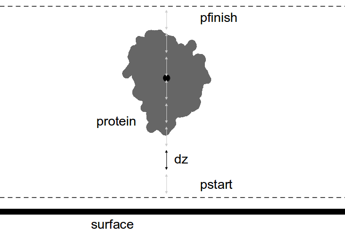
• Potential of mean force (PMF) calculations are based on a thermodynamic integration method where the configurational space of the solute with respect to a surface is sampled over the Euler angles (θ, ϕ, ω) and a number of dx,dy and dz coordinates based on the parameters:
• mentth [integer] (60) : Number of θ angles to be explored in rotational sampling. The angles range between 0 and π with a stepwise increment of (π ÷ (mentth - 1))
• mentfi [integer] (120) : Number of ϕ angles to be explored in rotational sampling. The angles range between 0 and 2π with a stepwise increment of (2π ÷ (mentfi - 1))
• mentom [integer] (60) : Number of ω angles to be explored in rotational sampling. The angles range between 0 and 2π with a stepwise increment of (2π ÷ (mentom - 1))
• mentx [integer] (6) : Number of subdivisions (dx) of the surface along the x axis to be sampled. The sampling length in the x direction is 6 Å
• menty [integer] (6) : Number of subdivisions (dy) of the surface along the y axis to be sampled. The sampling length in the y direction is 6 Å
• pstart [float] (0.0) : Starting distance of the center of geometry of the solute from the surface in Å
• pfinish [float] (60.0) : Finishing distance of the center of geometry of the solute from the surface in Å
• dz [float] (0.2) : Increment step (dZ) along the z axis in Å