Most of the tools are available in bin/ or bin_arch2/ after compilation, and the scripts are in the auxi/ directory. These tools are integrated into the SDA7 software, and use many classes defined in the library libsda.so.
However, a few programs have not yet been integrated and are only copies from SDA 6. Their source codes are in auxi/. When using these tools, be aware that they use a static allocation of memory and often define their own parameters (e.g. van der Waals radii).
Several examples of tools usage can be found in the folders with the exemplary runs.
If you need help, a full description of each tool with a list of arguments is provided by executing the program without any arguments!
- get_encounter_traj.sh: to select encounter trajectories from the trajectory and complexes files, and convert the ligand’s COG positions to xyz format in the target protein’s reference system.
- build_MSM.sh: to construct the MSMs of the encounter trajectories. Further information can be found in the README.md file located in the folder. The folder also contains a YAML file to create a Conda environment for running the Python scripts called by the two master Bash scripts.
This tool calculates the average and standard deviation from a single simulation and can be applied to:
- Association rate constant
- Electron transfer rate constant
- First passage time (under testing)
A simple implementation is used to obtain the standard deviation, it typically requires 100-200 resamples.
Its usage and advantages are demonstrated in the Barnase-Barstar association rate example.
The tool has dependencies on some python libraries (numpy and multiprocess).
There are 2 algorithms available for clustering the docking results:
- auxi/clust : an average-linkage algorithm
- auxi/k-mean.py : a K-Mean algorithm
More details are available on the Clustering page.
- extraction of energy terms and basic summary;
- conversion between ascii and binary formats;
- splitting of one file with complexes of the solute in different conformations into several files, one for each conformation;
- transformation of the 'new' complexes format into the old one, which can then be clustered further with the clustering utility provided;
- extraction of specific conformations from the complexes file;
- concatenation of several trajectories into one;
- extraction of specific frames from a trajectory file;
- extraction of configurations in which the two solutes are within a specified distance (only for trajectories recorded from the sda_2proteins type of simulation)
- conversion of the trajectory in the sdamm trajectory format used by sdamm
grid_input [ grid_output ], [-convert] / [ -scale factor ] / [ -dx ] / -exclude_molsurf pdb / [ -header_only ]The tool can convert grids between ascii and binary formats, modify their units (APBS output in kT units into kcal/mol units used by SDA for instance), to zero points inside the molecular surface of the solute (-exclude_molsurf) to facilitate simultaneous visualization of the solutes and their interaction field grids.
This tool estimates the diffusion coefficients of solutes in water at 293.15 K, using the Stokes-Einstein Law. The effective radius used in the calculation is taken as the radius at which the solute's atomic density is 2⁄3 times the atomic density at the centre. The bin size used for the density calculations can be set as an input parameter.
As this method is quite approximate, we advise the use of alternative methods (e.g. HYDROPRO), where possible.
In genbox, a user can request that a certain total number of molecules can be placed in a simulation box, with the cubic dimensions of the box, and the relative number of molecules of each solute type, calculated from the mass concentration of each solute. An example of an input file for such a calculation can be downloaded here. An immobile surface can also be included by setting the
surf flag to 1, and entering the surface as the final molecule type (as shown in the file above. In this case, the x and y
dimensions of the box will be fixed to those of the surface, and the simulated volume will be set by varying only the z dimension. Alternatively, a user can request that a box of fixed dimensions be filled with solutes at a fixed mass concentration. In this case, number of molecules of each solute type, and the total number of solutes, is calculated by the tool. An example of an input file for such a calculation can be downloaded here. In this case, including a surface is not currently supported.
In some cases, it may be desirable to simulate a fixed number of solutes of one molecule type within a fixed concentration of another. A fixed number of solutes of a certain molecule type can be added by setting its mass concentration (with the
dens option) to a negative number. In
cases where the box size is calculated by genbox, the fixed-number
solutes will be ignored when calculating the box size. Note that in
these cases, concentration
information must be supplied for at least one solute type, or the
box dimensions can not be calculated.By default, genbox is very conservative in avoiding solute overlaps when placing solutes. At high concentrations, it may be necessary to change the parameter
fit_factor
in the genbox input file to achieve the required solute
concentration. The parameter can be set to any value between 0.0 and
1.0. When fit_factor is set to
1.0 (its default), genbox is at its most conservative. When fit_factor
is set to 0.0, no checks for overlaps are made. When using a value
lower than 1.0, it is important to
check the early stages of the trajectory, to ensure that any
overlaps are removed during equilibration. It is best to choose the
highest value possible to achieve the desired
concentration, and only lower the value where necessary. A second parameter,
max_iter, sets the number of
times that genbox will attempt to place each solute in the simulation
box, while avoiding overlaps. This can be increased from its
default value of 5000 in the input file, although changing this alone
may still not allow the the desired concentration to be
reached, and it will increase the time required to run genbox.In genbox, there is an option to order the placing of solutes in the simulation by size, with larger solutes placed first. This can be turned on by setting the
sort option to 1. This may allow a better packing
of solutes, and allow a larger fit_factor to be used, but it can lead to strange packings, where all smaller solutes are placed near the box edge.- Electrostatic desolvation
- Nonpolar desolvation
- Soft-core repulsion (used for SDAMM only)
UHBD grids can be visualized directly with VMD, or converted into a DX for use with Pymol (convert_grid tool)
It can be run in a combined way as:
make_edhd_grid -ed ed.in -hd hd.in -ljrep ljrep.in-omit filename: Add this flag when the nonpolar desolvation potentials of the atoms listed in the file (pdb format) are to be neglected, e.g.:
make_edhd_grid -ed ed.in -hd hd.in -ljrep ljrep.in -omit atoms.pdbThis option may be useful for computing association rates for small molecules.
This code is parallelised with OpenMP.
ed.in, has the following format:
	#------------------------------ h,ndimx,ndimy,ndimz

	1.0, 110,110,110

	#------------------------------ iostr,epssol,rion

	100.  78.  2.0

	#------------------------------ pfile

	pqrnoh_h5a.pdb

	#------------------------------ efile, iform

	h5a_ed.grd

	0
Here, the first 4 parameters give the electrostatic desolvation grid
spacing (Å) and the grid dimensions along the x,y,z axes. The second set
of parameters describe the ionic strength (mM), solvent dielectric
constant and ion radius (Å) relevant for defining the ionic strength
conditions. Note that, depending on the grid multiplication factor used
in the sda input file, in may be necessary to set the ionic strength (iostr)
to zero, (for details, see "Multiplicative factors applied to the
grids" in the "Description of input files"). Next, the name of the PDB
file to read from is given. The last parameters are the name of the
output file containing the grid and whether it should be in binary (0)
or ascii (1) format.
hd.in, the format is similar:
	#------------------------------ h,ndimx,ndimy,ndimz

	1.0, 75, 75, 75

	#------------------------------ a,b,factor

	3.10, 4.35, 0.5

	#------------------------------ pfile

	pqrnoh_h5a.pdb

	#------------------------------ efile, iform

	h5a_hd.grd

	0
The first set of parameters is identical to the ed.in
file. The second set of parameters specifies the region where this
potential is defined and the scaling factor for the calculated
potential.This procedure assigns a value of gamma (parameter "factor" in the input file above) to all points within distance a (in Å) from the surface of the solute, zero if a point is further than b (in Å) from the surface and a linearly interpolated value if a point is in between a and b:
In SDA, the solvent accessibility values of the atoms of one solute are multiplied by the nonpolar desolvation values of the other solute. As shown in the plot below, there are several different values of parameters a and b that give the buried areas to an accuracy of ca 10%. We recommend using the values: a =3.10, b = 4.35, and factor = 0.5.
ljrep.in, is required for the
SDAMM-type of simulation, and optional for two solute simulations (where
repulsion is normally modelled using excluded volume checks):
	#------------------------------ h,ndimx,ndimy,ndimz

	1.0, 60,60,60

	#------------------------------ factor, nexp, fraction

	4096.d0, 6, 1.5d0

	#------------------------------ pfile

	prqnoh_h5a.pdb

	#------------------------------ efile, iform

	ha5_ljrep.grd

	0
The potential is of the form:
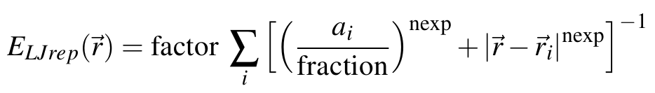
where summation is over all atoms of the solute, and r_i and a_i are the position of the center and the radius of atom i, respectively. The value of fraction can be tuned to vary the smoothness of the function, while the nexp value defines the decay.
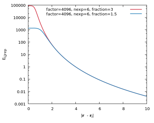
The plot above shows the value of the repulsive potential at distances (Å) from a single atom of radius a = 1.8 Å for two parameterisations that have been used in SDAMM publications (see Mereghetti et al. (2010) for the parameterisation of the red potential, and Mereghetti and Wade (2011) for the blue. Note that the ultimate interaction energy between a pair of solutes (See Equation A8) depends also on the value of lj_rep_fct defined in the input file used during SDA simulations, with the product of factor and lj_rep_fct giving γ in Equation A9. With both of the parameterisations shown in this plot, lj_rep_fct = 0.0156 should be used.
rxna2rxnaC p1.rxna p2.rxna [outFileName] [dist] [specificity]Where p1.rxna and p2.rxna are the output files from the nda-pairs tool. Optionally, it is possible to specify the filename of the output file (default: p12.rxna), the cutoff distance for the reaction pairs (default: 6 Å) and the type of criteria (specificity (=0) or nonspecific (=1), default: 1)
python holo2apo.py -apo [apopdb] -holo [holopdb] -rxna [rxnafile]The output filename is saved as p2.rxna
python rm_highflex_residues.py -pdb1 [pdbFilename] -rmsf [rmsfFile] -rxna [rxnaFile] -o [outputFilename]However, if a second pdb is provided rather than RMSF values, the script will superimpose the two pdbs to calculate the RMSD of the residues, and remove from the reaction criteria list the residues with an RMSD greater than 4.0 Å.
python rm_highflex_residues.py -pdb1 [pdbFilename] -pdb2 [pdbFilename] -rxna [rxnaFile] -o [outputFilename]It is also possible to indicate if the protein is symmetric with the -prot_symm argument (Options: yes/no; Default: no). When this option is enabled, the script identifies symmetric counterparts of the protein residues (e.g. if one solute is a protein homodimer). Then, it will exclude these symmetric residues from the reaction criteria if either of the symmetric parts has an RMSD or RMSF value greater than 4.0 Å.
This code is parallelised on one compute node and uses by default all available cores. To limit this, you can set the environment variable OMP_NUM_THREADS to the desired number. Also you might need to increase the stackspace by setting ulimit -s 1000000.
The program prepLJgrids.py calls three other scripts-
auxi/LJ-GRID-preparation/change_atomNames.sh, auxi/LJ-GRID-preparation/PrepareProbeFile.py, and auxi/LJ-GRID-preparation/mk_LJ_grd:change_atomNames.sh- fixes atom names in a protein pdb file according to the OPLS format;PrepareProbeFile.py- assignes Lennard-Jones parameters to each type of the probe (gold atom, 2 types) and protein atoms. Output file is "ProbeFile.txt".mk_LJ_grd- generates Lennard-Jones grids for each probe type (i.e. grids for Au(111) surface in GolP force field) using "ProbeFile.txt" as an input.
prepLJgrids.py:
- pdb files for a protein and a surface
- opls database containing Lennard-Jones parameters of OPLS and GolP force fields (
qtable_Parameters_30_10_09.dat) - input file
prepLJgrids_inputwith parameters of the grid to be simulated and with additional Lennard-Jones parameters for interaction of specific groups (for example, aromatic rings) with gold.
prepLJgrids_input:
	#optional parameter - grid step size in A, default value is 0.2 A (the optimal value is <0.3A)

	h	0.2

	#optional parameters - grid size in A, in x,y and z direction (the optimal value can be defined as (protein_size+20)/h

	ndimx	300

	ndimy	300

	ndimz	300

	#essential parameter - filename of the protein structure in PDB format

	pfile	p2.pdb

	#optional parameter - filename of the LJ Grid, note that some prefix is added by the mk_LJ_grd_executable

	efile	LJp2

	#optional parameter - format of the LJ Grid. 1=ASCII,0=BINARY. Default value is 1

	iform	0

	#optional parameter - filename of the output probefile which is created by PrepareProbeFile_executable

	probef	ProbeFile.txt

	#optional parameter - default 0. If 1 more output is generated by the mk_LJ_grd_executable.

	ioset	0

	#optional parameter - at distance larger then the cutoff the energy is set to zero. default value 10A

	cutoff	10

	#essential parameter - filename of the suface structure in PDB format

	#SurfaceFile gold_3layers.pdb

	SurfaceFile  gold3layersflex.pdb

	#essential parameter - filename of the qtable

	ParameterFile qtable_Parameters_30_10_09.dat

	#optional parameter - name of the inputfile which is used as the input
for mk_LJ_grd_executable. This file is created automatically, no need to
 change this parameter.

	LJinput lj2.in

	#optional parameter - At small distance from the atom (r <
sigma_ii/2) the energy equals OVERLAPENERGY. default value is 1.e1
kcal/mol

	OVERLAPENERGY 1.e1

	#  Optional parameter: executable  file for calculation of the LJ-grid

	#mk_LJ_grd_executable ../../../bin/mk_LJ_grd

	############### ADD ADDITIONAL PROBES AS IN THE ProbeFile Format from
the PrepareProbeFile_executable KEYWORDS: PROBE,INTERACT
###############################

	PROBE Av_CEN

	INTERACT ND1_HIE 2.75 0.3824  # name sigma epsilon

	INTERACT SG_CYS  2.0 0.6


	INTERACT CG_TYR 3.37045990927 0.148089  # name sigma epsilon

	INTERACT CD1_TYR 3.37045990927 0.148089  # name sigma epsilon

	INTERACT CD2_TYR 3.37045990927 0.148089  # name sigma epsilon

	INTERACT CE1_TYR 3.37045990927 0.148089  # name sigma epsilon

	INTERACT CE2_TYR 3.37045990927 0.148089  # name sigma epsilon

	INTERACT CZ_TYR 3.37045990927 0.148089  # name sigma epsilon


	INTERACT CG_TRP 3.37045990927 0.148089  # name sigma epsilon

	INTERACT CD1_TRP 3.37045990927 0.148089  # name sigma epsilon

	INTERACT CD2_TRP 3.37045990927 0.148089  # name sigma epsilon

	INTERACT CE2_TRP 3.37045990927 0.148089  # name sigma epsilon

	INTERACT CE3_TRP 3.37045990927 0.148089  # name sigma epsilon

	INTERACT CZ2_TRP 3.37045990927 0.148089  # name sigma epsilon

	INTERACT CZ3_TRP 3.37045990927 0.148089  # name sigma epsilon

	INTERACT CH2_TRP 3.37045990927 0.148089  # name sigma epsilon


	INTERACT CG_PHE 3.37045990927 0.148089  # name sigma epsilon

	INTERACT CD1_PHE 3.37045990927 0.148089  # name sigma epsilon

	INTERACT CD2_PHE 3.37045990927 0.148089  # name sigma epsilon

	INTERACT CE1_PHE 3.37045990927 0.148089  # name sigma epsilon

	INTERACT CE2_PHE 3.37045990927 0.148089  # name sigma epsilon

	INTERACT CZ_PHE 3.37045990927 0.148089  # name sigma epsilon


	INTERACT CG_HIE 3.37045990927 0.148089  # name sigma epsilon

	INTERACT CD2_HIE 3.37045990927 0.148089  # name sigma epsilon

	INTERACT CE1_HIE 3.37045990927 0.148089  # name sigma epsilon


	PROBE Au_CEN 002

	INTERACT ND1_HIE 2.75 0.3824  # name sigma epsilon


	INTERACT CG_TYR 3.37045990927 0.104169  # name sigma epsilon

	INTERACT CD1_TYR 3.37045990927 0.104169  # name sigma epsilon

	INTERACT CD2_TYR 3.37045990927 0.104169  # name sigma epsilon

	INTERACT CE1_TYR 3.37045990927 0.104169  # name sigma epsilon

	INTERACT CE2_TYR 3.37045990927 0.104169  # name sigma epsilon

	INTERACT CZ_TYR 3.37045990927 0.104169  # name sigma epsilon


	INTERACT CG_TRP 3.37045990927 0.104169  # name sigma epsilon

	INTERACT CD1_TRP 3.37045990927 0.104169  # name sigma epsilon

	INTERACT CD2_TRP 3.37045990927 0.104169  # name sigma epsilon

	INTERACT CE2_TRP 3.37045990927 0.104169  # name sigma epsilon

	INTERACT CE3_TRP 3.37045990927 0.104169  # name sigma epsilon

	INTERACT CZ2_TRP 3.37045990927 0.104169  # name sigma epsilon

	INTERACT CZ3_TRP 3.37045990927 0.104169  # name sigma epsilon

	INTERACT CH2_TRP 3.37045990927 0.104169  # name sigma epsilon


	INTERACT CG_PHE 3.37045990927 0.104169  # name sigma epsilon

	INTERACT CD1_PHE 3.37045990927 0.104169  # name sigma epsilon

	INTERACT CD2_PHE 3.37045990927 0.104169  # name sigma epsilon

	INTERACT CE1_PHE 3.37045990927 0.104169  # name sigma epsilon

	INTERACT CE2_PHE 3.37045990927 0.104169  # name sigma epsilon

	INTERACT CZ_PHE 3.37045990927 0.104169  # name sigma epsilon


	INTERACT CG_HIE 3.37045990927 0.104169  # name sigma epsilon

	INTERACT CD2_HIE 3.37045990927 0.104169  # name sigma epsilon

	INTERACT CE1_HIE 3.37045990927 0.104169  # name sigma epsilon
Grid files with DT-Grid format can safely be input to SDA when created using the UHBD2dtgrid tool (see below).
SDA determines the type (UHBD or DT-Grid) of an input grid internally from its contents.
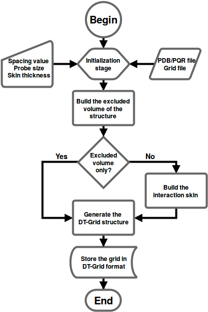
The program reads the interaction grid (created beforehands) of a molecule along with a structure file (PDB or PQR).
In case of an excluded volume grid, no input grid file is required. The program calculates the excluded volume and stores directly in DT-Grid format.
The workflow the UHBD2dtgrid program is shown below:
USAGE:
./UHBD2dtgrid -g uhbd.grd -p protein.pdb -f binary [-other options]
Options:
-g : The UHBD file name to be converted into DT-Grid
-p : The PDB file name to be used to generate the molecular skin
-f : The output file format. There are two options: Binary and ASCII. You can save your DT-Grid using the format you want
-o : The name of the outputting *.dtgrd file name. The grid file will be named as 'dt.dtgrid' unless this option is used
-s : The thickness of the skin around the surface of the molecule. A default value of 2.0 Angstrom will be used unless this option is used
-sp : The spacing required to build the exclusion grid. A default value of 0.5 Angstrom will be used unless this option is used
-pr : The size of the probe used to compute the molecular skin. A default value of 1.7 Angstrom will be used unless this option is used
-type : Type of grid: exclusion grid (0), normal grid (1). Default value is 1. No UHBD file is required for an exclusion grid
-h : Displays the usage information and terminates the execution!
Note that not all information will be recovered as the grid points that lie outside the interaction field will store a constant value provided by the user upon conversion to UHBD format!
USAGE:
./dtgrid2UHBD -g dt.dtgrd -f binary [-other options]
Options:
-g : The DT-Grid file name to be converted into UHBD
-f : The output file format. There are two options: Binary and ASCII. You can save your UHBD using the format you want
-o : The name of the outputting *.grd file name. The grid file will be named as 'dtgrid2.uhbd' unless this option is used
-v : The number used for omitted values during the conversion from UHBD to DT-Grid. A default value of 0.0 will be used unless this option is used
-excl : Input DT-Grid is of type exclusion. Grid is assumed to be a data grid, if this option is not used!
-h : Displays the usage information and terminates the execution!
sdamd = 1 in the input file to enable suitable output from the BD trajectories for the subsequent MD simulations.See auxi/Kon-rates-SmallMolecule/Generate-ECMSites-SmallMol/usage.pdf for documentation.
See auxi/Kon-rates-SmallMolecule/Generate-ReactionCriteria/usage.pdf for documentation.
The tool can be found in the auxi/sdamd directory sdamd.sh. An example of how to use it can be found in the README file.
The tool can be found in the auxi/convert-to-browndye directory. An example on how to use it can be found in the examples section.
An example of use convert_sda_to_browndye.sh can be found in README
The AMBER software can be downloaded here