|
SDA (SDA flex)
7.2
Simulation of Diffusional Association
|
|
SDA (SDA flex)
7.2
Simulation of Diffusional Association
|
The functionalities from SDA 6 and SDAMM have been unified into a single codebase, making it easier to develop new functionalities for either or both codes.
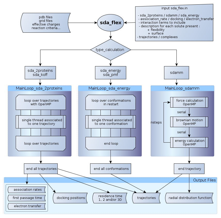
The following calculations are possible for two-solute simulations only (comparable to SDA 6 simulations):
For multiple solute simulations up to high concentrations: (formerly in SDAMM)
For solute diffusion to surfaces:
The following interaction types are implemented:
New features :
SDA 7 is written in Fortran 90. The additional features of Fortran 90 allow for a more "object oriented design" for the software than was possible with Fortran 77 which was used for previous versions of SDA.
The main new feature of SDA 7 is the introduction of 'flexibility' for one or all of the solutes. Flexibility is introduced by considering several rigid body representations of a protein taken from an NMR ensemble, molecular dynamics simulation, normal mode analysis, or another relevant conformational sampling technique. SDA 7 can then swap between these representations based on e.g. a Monte Carlo criterion. Thus multiple conformations can be treated within a single trajectory.
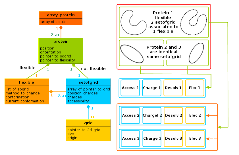
The diagram below: "Diagram of Solutes, Grids and their relationship", shows the relationships between key modules and how multiple solutes and flexibility are implemented:
In the diagram solute 1 is flexible, and has two possible conformations. During the trajectory, solute 1 changes conformation, from conformation 1 to conformation 2 (algorithms are discussed below). The change in conformation is performed by changing the association of the pointer (p_current_node) of the flexible object to the setofgrid for the conformation
Solutes 2 and 3 are identical solutes and are not flexible. As they are not flexible, flexible objects do not need to be created.
The solutes are identical, therefore they are directly associated with a single setofgrid, resulting in efficient use of memory. Only the positions and orientations of solute 2 and 3 must be stored independently.
It is straightforward to specify many identical flexible solutes: All solutes are associated to their own flexible object, associated to their current conformation. They all share the same possible conformations, defined by N setofgrid.
The design presented is efficient for the memory usage, but has one important limitation:
The compromise made in SDA (since its origin in 1998) is to apply these rotations at every step, when the Brownian Dynamics update is applied in make_bd_move. Only the rotation is applied, not the translation. The translation is indeed recomputed each time that the instantaneous position of a movable atom is needed. The full transformations (rotation and translation) are required at several stages, e.g. for computing the interactions, checking overlap with the exclusion grid, checking reaction criteria, etc., and many other functionalities. There were many reasons to use this implementation in SDA 6 (and previous versions): Only two solutes were simulated and the larger solute, solute 1, is kept fixed throughout the simulation, so this transformation was needed only for the smaller, second solute.
Different parallelisation schemes are used in SDA 7. To help understand the parallelisation schemes, we briefly discuss each simulation type, and then the strategy used for parallisation with some pseudo codes.
In SDAMM simulations, only one trajectory is generated and the trajectory has a predefined number of steps. The most computationally expensive subroutines are :
The method of parallelisation is a straightforward application of OpenMP, with the main loop split between threads in these specific subroutines. For the force and energy calculations:
      do s1 = 1, n
         do s2 = s1 + 1, n
            interaction12, interaction21 = compute_interaction_between_solute1_and_solute2()
            total_interaction ( s1 ) = interaction ( s1 ) + interaction12
            total_interaction ( s2 ) = interaction ( s2 ) + interaction21
         end do
end do !$OMP PARALLEL
!$OMP REDUCTION(+:all_interaction)
!$OMP DO SCHEDULE( DYNAMIC )
do s1 = 1, n ! only the first loop is split over the threads
do s2 = s1 + 1, n
interaction12, interaction21 = compute_interaction_between_solute1_and_solute2()
! secure because of REDUCTION
total_interaction ( s1 ) = interaction ( s1 ) + interaction12
total_interaction ( s2 ) = interaction ( s2 ) + interaction21
end do
end do
!$OMP END DO
!$OMP END PARALLELThe implementation of the parallelisation with two solutes is very different from that for SDAMM:
The approach chosen for parallelisation is to split the total number of trajectories across the different threads. Each thread is responsible for running a full trajectory. When one trajectory is finished, the thread will start calculating a new trajectory, until no more trajectories need to be conducted.
The difficulties with this approach are:
      !$OMP ATOMIC
      global( i ) = global ( i ) + local ( i )
    MainLoop( tab_protein_unique )
    !$OMP PARALLEL
    ! allocate local array, OpenMP or not
    allocate ( local_escape, local_sumtime,...)
    ! if OpenMP make a copy of the Solutes
!$  if ( tid > 0 ) then
    !$      call copy_array_protein ( tab_protein_unique, ptab_protein, type_calc )
    ! normal if not OpenMP or master
!$  else
        ! write (*,*) 'Associate ptab_protein to tab_protein_unique'
        ptab_protein => tab_protein_unique
!$  end if
    ! if OpenMP make a local copy of the list of complexes ( here empty, only copy data members )
!$  if ( tid >= 0 )  then
!$      call copy_record ( o_complexes, p_local_complexe, .false., size_thread_complexe )
    ! else normal if not openMP
!$  else
        ! associate the global pointer to o_complexe if not openmp
        if ( associated ( o_complexes % pcomplexe ) ) then
            p_local_complexe => o_complexes
        end if
!$  end if
    ! not necessary but convenient, simpler to refer to solute 1 and 2
    protein1 => ptab_protein % array ( 1 )
    protein2 => ptab_protein % array ( 2 )
    !$OMP BARRIER
    !$OMP DO SCHEDULE( DYNAMIC )
LOOP_RUN: &
    do run = 1, total_traj
       !$ if need to merge complexes every 100 runs
          !$OMP CRITICAL ( crit_merge_p_complexe )
          !$      call merge_complexe ( o_complexes, p_local_complexe )
          !$OMP END CRITICAL ( crit_merge_p_complexe )
       !$ endif
       call init_position_protein()
       ! begin BD loop
LOOP_STEP: &
       do
           call force_epedhdlj_2proteins_fast( protein1, protein2 )
           call make_bd_move_2prot( protein1, protein2 )
           call check_reaction_pairs( protein1, protein2 )
       ! add to the list of complexes
           if ( complexe_to_record .eqv. .true. )
               call energy_epedhdlj_2proteins_fast( protein1, protein2, energy )
               call add_record ( p_local_complexe, ptab_protein % array ( 2:2 ), energy )
              end if
           ! use atomic inside
           call update_residence_time ( resid_time, protein2 % position, dist, dtnow )
       end do LOOP_STEP
       ! only at the end of the trajectory
       call update_escape()
   end do LOOP_RUN
   ! deallocate Solutes for all threads, except the MASTER
   nullify ( protein1, protein2 )
!$ if ( tid > 0 ) then
       !option true for NOT deleting the grid
!$     call delete_array_protein ( ptab_protein, .true. )
       ! now need explicit deallocation of the pointer
!$     deallocate ( ptab_protein,  stat = ierr )
!$     nullify ( ptab_protein )
!$ end if
    ! same deallocation for local_complexes
The use of OpenMP pragma allows a compilation with or without OpenMP (without loss of performance). With this implementation a high level of parallelization is achieved because there is no sequential code in the main loop. The merging of the lists of complexes is still the main limitation, but their frequency can be tuned for a specific system and computer architecture.
A demonstration simulation with 6 trajectories and 3 available threads can be represented by the scheme below
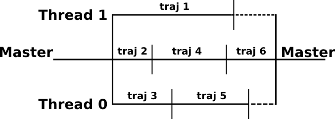
Each thread runs calculations for one trajectory. When a trajectory is completed, the thread will run the next trajectory. At the very end of the calculation there are no more trajectories to perform and N-1 CPUs are in a waiting state. This may be a problem for association rate calculations where trajectories can, in principle, last for an infinite amount of time. In practice this effect is usually minor.
It is difficult to estimate the end effect during runs to test the performance of SDA 7 (relatively short runs with X trajectories, where X is generally small ~ 100), so the scaling is generally underestimated compared to that expected for a real simulation (> 10,000 trajectories).
In the most favorable case, association rates calculations (with no complexes recorded) have scaling reaching 80 % on 48 CPUs.
The implementation of computations of forces and of energies are similar in sda_2protein and SDAMM, but they are nevertheless implemented in different functions for optimization. The differences are the double-loop over all pairs of solutes in the case of SDAMM (as seen in the parallel section) and the fact than the first solute is always kept fixed in sda_2proteins.
In the following sections, we use the example of the computation of the energy of the charges on solute 1 in the potential grid of solute 2.
The following five types of interaction are described as "charges" interacting with a potential grid.
The other energy terms: metal desolvation, and the correction to the image-charge have a different implementation and will not be considered in this section.
All energies are computed as :
\[ E_{12} = \sum_{i=1}^n q_1^i(x,y,z) \, U_2(x,y,z) \]
where \(E_{12}\) is the energy of the effective charges from solute 1, \(q_1\), in the potential of solute 2, \(U_2\).
With the exception of the electrostatic energy, the total energy is evaluated as the sum of those components, \(E = E_{12} + E_{21}\).
For the electrostatic interaction energy, the definition is slightly different. The total electrostatic energy should satisfy:
\[ E_{el} = E_{12} = E_{21} \]
But due to approximations in the electrostatic potential grid and effective charges computations, the results of \(E_{12}\) do not exactly equal \(E_{21}\). In order to use the same algorithm for each type of interaction, we estimate the total electrostatic energy as the average of the two components:
\[ E_{el} = \frac{1}{2} ( E_{12} + E_{21} ) \]
Where the factor \(\frac{1}{2}\) is applied on the electrostatic potential grids when they are read into memory. It can be adjusted in the SDA7 input file with the parameter epfct (default 0.5)
The same applies for the forces, with the difference that we need the derivatives of the energy:
\[ \vec{f_{12}} = \sum_{i=1}^n - \, q_1^i(x,y,z) \, \nabla U_2(x,y,z) \]
The values of the energy and the derivatives are extrapolated from the grids (see functions mod_force_energy::potential_atom_uhbd and mod_force_energy::force_atom_uhbd ). Note that pointers to the grids are used, rather than the original grid. The use of pointers allows for these functions to be used on any 3-dimensional grid of real*8. It is therefore relatively straightforward to implement calculations of new energy and force terms.
All grids and charges have a type associated with them (enumerated in mod_gridtype), all grids derive from the same class mod_grid. The types are used to select the correct association between charges and grids. This is performed by the function mod_protein::select_charge. Given the grid_number, the mod_protein::select_charge function associates pointers to the charges and the grids. Pointers are then used for computing the interactions by the same subroutine. A simple and general method for evaluating the forces is summarized here schematically. It is simplified pseudo-code, from mod_compute_force::force_epedhdlj_2proteins, which does not take into account asymmetric interactions.
   subroutine energy_epedhdlj_2proteins ( prot1, prot2,...)
       ! loop over grid, sure to be associated because a pre-sorting is done in param_force_energy
GRID:  do i = 1, param_force_energy % nb_grid
         ! extract the grid number, identical to accessing the sogrid directly
         grid_number =  param_force_energy % array_grid_calc ( i, 1 )
         call compute_force_sda_2proteins ( prot1, prot2, grid_number,..)
       end do
   end subroutine

   subroutine compute_energy_sda_2proteins ( prot1, prot2, grid_number,..)
       ! assign correctly the pointers from the grid_number
       call select_charge ( grid_number, prot1, prot2, nq1, nq2, p_charge1, p_charge2, &
                            p_charge_position1, p_charge_position2, dummy_array )
       ! compute force, discussed in detail the next chapter
       Energy 12 = Sum of p_charge1 * U ( p_charge_position1, prot1 % p_sogrid % pset ( grid_number ) )
       Energy 21 = Sum of p_charge2 * U ( p_charge_position2, prot2 % p_sogrid % pset ( grid_number ) )
end subroutineThere are several possible methods for calculating the force (and energy), here we present the simplest one. Its advantage is, as its name suggests, simplicity, and in addition generality. This method should be used as the first when a new type of interaction is being added to the code, since it greatly reduces the risk of introducing errors. The principal difficulty is dealing with the coordinate transformation between frames of reference, because the grids are fixed and never rotated.
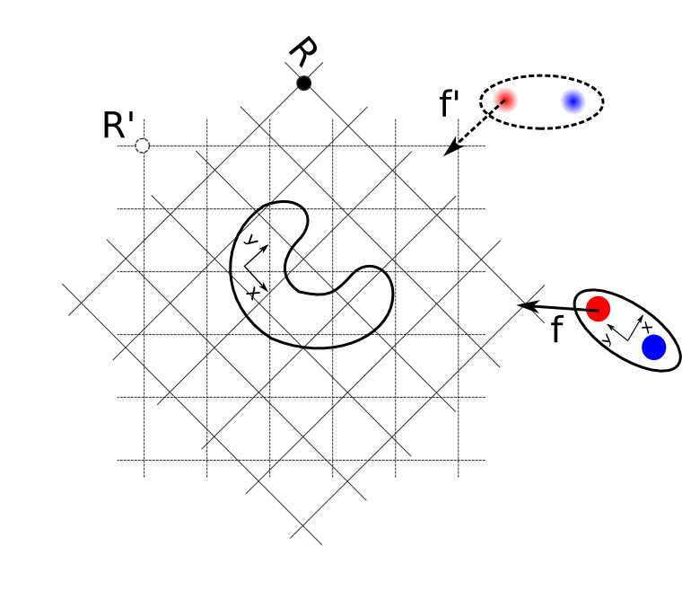
The figure "Computation of forces" shows the general computation of \(f_{21}\), the force applied on solute 2, when both solutes can rotate (e.g. the case of SDAMM).
The solute 1 grid shown with the dashed line represents the grid orientation in the fixed frame of reference R', and is stored in memory. The solid lines represents the grid orientation corresponding to the instantaneous orientation of solute 1 (frame R).
The simple algorithm is a loop over the charges of solute 2:
 subroutine compute_force_sdamm_2proteins( prot1, prot2, pos_relat,..)
    ! get the orientation of the first solute
    ex = prot1 % orientation_x
    ey = prot1 % orientation_y
    ez = prot1 % orientation_z
    ! inverse the matrix, it is a unity matrix : transposed equal the inverse
    xe(1) = ex(1)
    xe(2) = ey(1)
    xe(3) = ez(1)
    ye(1) = ex(2)
    ye(2) = ey(2)
    ye(3) = ez(2)
    ze(1) = ex(3)
    ze(2) = ey(3)
    ze(3) = ez(3)
! loop over the charges of solute 2
FORCE2: do j=1,nq2
        ! pos_relat is the relative position of the center of geometry of the solutes, and p_charge_position2 have the correct orientation
        p2 = p_charge_position2 (:,j)
        ! relative position of the charge in the frame of reference R
        rto = p2 + pos_relat
        ! make the trnasformation between the frames of reference, rtn is the relative position in the frame R'
        call tr ( rto, rtn, ex, ey, ez )
        ! get the derivative of the potential at the position rtn
        call force_atom_uhbd ( rtn, force, prot1 % p_sogrid % pset_grid ( grid_number) )
        ! transform back into R
        call tr ( force, force_o, xe, ye, ze )
        ! multiply by the charge to get f in R. Back transformation and multiplication can be inverted here
        qf = force_o * p_charge2(j)
        ! call the cross product to get the torque, directly in R
        call cross (tmp2, p2, qf )
        ! add to the total torque and force
        tt2 = tt2 + tmp2
        ff2 = ff2 + qf
    end do FORCE2
With the code presented, we could compute all interactions, both for sda_2proteins and SDAMM.
There are nevertheless different implementations for optimizing the calculations. In sda_2proteins, solute 1 is always fixed, so that some computations are simpler: the charges of solute 2 remain in the reference frame.
Two improvements of the simple algorithm are made:
The functions that implement these improvements have an equivalent name to the functions implementing the simple algorithm, with the "fast" suffix added. The module mod_force_energy stores alot of information about the required calculations. In particular, where beneficial, it uses the optimized (i.e. fast) functions.
The fast algorithm is more difficult to maintain than the simple algorithm, but in the best case (SDAMM with all four interactions) there is a 50% gain in performance.
SDA 7 has three output file types which are used to store the positions and orientations of solutes, along with energy information. Complex files are used to store the docked positions of the mobile solute, relative to the fixed central solute, obtained from docking simulations. Trajectory files may be generated from either two solute or many solute simulations. In two solute simulations, there are used to store trajectories of the mobile solute relative to the fixed solute, while in many molecule simulations they show the trajectories of all solutes, in the frame of the simulation box. Finally, restart files can be used to restart many molecule simulations from the end of a previously run simulation. They have the same form as a single frame from a trajectory file.
The the form of these output files has been changed, compared to SDA6. The specifications for the new design were :
A versioning has also been included to maintain compatibility with previously generated files, should new formats be added.
The requirements cited above apply to both complex and trajectory files. Their functions are indeed very similar: they record information about the solutes (solute number, conformation number...), the solute's position and orientation, the energy interactions terms and additional statistics dependent on the type of simulation. However their use differs. New data for trajectory files is always appended to the file each time it is written, to give a chronological order to the file. On an other hand, complex files are ordered by the energy values of the recorded complexes. The best complexes (with the lowest interaction energy) are at the top of the file, while those with the largest interaction energies not stored, this gives the maximum number of relevant complexes, which can be analysed later with external tools, such as clustering algorithms.
The implementation of the complex and trajectory files in SDA 7 groups the similarities into a main class record. All the functions/tools that use complexes and trajectories objects, should call functions from record.
Moreover, each "line" of these files is defined in the class one_complex (it's called 'complex' but it refers to one solute).
The main difference between complexes and trajectories files is in the implementation of intermediate types: ListComplexes and Trajectory. There are different algorithms for collecting the objects of type one_complex into complexes and trajectories:
The scheme below shows a schematic design of those modules: The information stored in each one complex can vary but it always follows the same order:
The information about what is written to disk in each file is coded in the header of the complexes/trajectories file (defined in description_column_str), if these are in ascii format. The header contains all information to read the following lines. It is constructed in header_str or directly printed from write_header_bin, and is composed of:
The five mysterious integer values present in the header describe the following options:
The first 2 integers are read and written as bits. The idea was to store the information about the presence of a term or not and avoid repetitive numbers.
The implemented solution uses the binary representation of those integers as logical values. As an example of bit_energy, the value of 5 in binary representation is written as:
       5
     00000101 <- we have to read from the right to the left
T
his value codes the following information (remember that the order of the terms is fixed):
      14
     00001110
Which means that:
Which means that:
In principle, all the classes using the complexes/trajectories, should use the interface functions implemented in mod_record and mod_onecomplexe, and not deal directly with the BITS functions themselves!
Below, we show a very simple exemplary code. Real examples can be found in tools (specifically in read_record.f90 and in trajectory2dcd.f90).
The code reads an existing record (complex or trajectory), extracts useful information and writes the new complexes or trajectory file to the disk.
    ! simple initialization, nullify pointers. clean for allocated objects
    call init_record ( o_record, opt_iocmx = io_record )
    ! read complex or trajectory (information in header), ascii or binary
    ! set all internal fields and bits from the header
    ! if optional nb_line, count the number of lines and assign it to nb_line
    call read_header_record ( in_record, filename, cm, nb_line )
    ! finalize a correct initialization, optional .true. do not write the header
    call initialize_record ( o_record, tab_prot, .true. )
!!!!!!!!!!!! Read data
! can read all data at once
    ! for traj can proceed by steps or multiple of steps
    call read_file_record ( o_record )
    ! reset position, complexe or trajectory
    call reset_position ( out_record )
! can loop over each one_complexe's
    ! p_tmp_onecomplexe is a convenient shortcut (for o_record % p_onecompl),
    ! will be updated with the getNext optional argument
    p_tmp_onecomplexe => o_record % p_onecompl
    ! make a loop over all entries
    do while ( ( ierr == 0 ) )
        ! if correctly set_up applies for sda 2proteins and sdamm
        do i = 1, nb_prot_in
             !!!!!!!!!!!!!!!!!!!!!!!!!!!!!!!!!!!
             !! Here make whatever you want
                !!! Read input
                ! e.g., get the conformation number, method 1 with indice_nconf data member of record
                if ( iflex ) then
                    tmp_conf = p_tmp_onecomplexe % int_ocompl ( o_record % indice_nconf )
                end if
                ! get integer and energy information from the current one_complexe
                ! order is natural : 4 integer, as many as necessary real
                call return_compatible_array_wrap ( o_record, array_int, array_real, other_real )
                ! e.g., get position and orientation
                !
                ! Here need to declare tab_prot explicitely before, see example in trajectory2dcd.f90
                tab_prot % array ( tmp_prot ) % position = p_tmp_onecomplexe % position
                tab_prot % array ( tmp_prot ) % orientation_x = p_tmp_onecomplexe % orient_x
                tab_prot % array ( tmp_prot ) % orientation_y = p_tmp_onecomplexe % orient_y
                !!! Write output
                ! allocate onecomplexe, with different fileds (coming from record_comp)
                allocate ( p_new_onecomplexe, stat = ierr )
                call new_onecomplexe ( p_new_onecomplexe, record_comp % nb_int, record_comp % nb_real, record_comp % nb_other_real )
                call set_onecomplexe_wrap ( record_comp, p_tmp_onecomplexe % position, p_tmp_onecomplexe % box, &
                                    p_tmp_onecomplexe % orient_x, p_tmp_onecomplexe % orient_y, &
                                    array_int, array_real, other_real, opt_p_onecomplexe = p_new_onecomplexe )
                ! always insert onecomplexe at the end
                call insert_new_node ( record_comp % pcomplexe % p_last, p_new_onecomplexe )
             !!!!!!!!!!!!!!!!!!!!!!!!!!!!!!!!!!!!
             ! go to the next one_complexe
             ! optionaly increment p_tmp_onecomplexe to the next element
             call getNext(  record_traj, p_tmp_onecomplexe, ierr )
         end do ! loop over solutes
         ! or write the data here in case of sdamm, after having read all solutes
         ! increment the loop
         nloop = nb_line + 1
    end do ! loop over nb_line
    ! clean memory from the record
    call delete_record ( o_record, .true. )
    ! write output into disk and clean the memory
    call write_record ( record_comp, .false. )
call delete_record ( record_comp, .true. )We have tested SDA 7 compilation on Linux with:
We had errors during the link stage with a MacOS (maverick XOS with gfortran 4.8). In the provided Makefile, the default options for the intel compiler (-warn all) are very strict.
The declaration of interfaces (for all the functions not contained in a given module) is mandatory in this case. Fortran does not use header files, so without those interfaces it is impossible for the compiler to notice a wrong or even missing argument of a function. It is convenient to check the integrity of the code, and may save (a lot by experience) debugging time.
SDA 7 uses extensive memory allocation. It requires explicit allocation of and deletion of objects from the heap memory.
Valgrind ( http://valgrind.org/ ) has been used during the development of the software. It is invaluable for finding mistakes (forget to free memory) or bugs (writing outside an array) in the code.
In 90 % of the cases, it answers the question (and gives the origin of the error if the code was compiled with "debug=yes" option): Why does my program crash on the cluster? It was working fine on my workstation!!
We recommend to use this tool when modifying the SDA7 code or developing a new module/tool to avoid accumulation of mistakes and errors. The released version gives 0 errors and 0 memory leaks in the serial version, when compiled with gfortran (as far as tested), however there are a few errors related to the use of OpenMP when using Valgrind.
When compiling with the intel compiler, more errors are found by Valgrind, many related to the use of SSE instructions.
 1.9.8
Imprint/Privacy
1.9.8
Imprint/Privacy